tfsmoment
Conditional spectral moment of the time-frequency distribution of a signal
Syntax
Description
Time-frequency moments provide an efficient way to characterize signals whose frequencies change in time (that is, are nonstationary). Such signals can arise from machinery with degraded or failed hardware. Classical Fourier analysis cannot capture the time-varying frequency behavior. Time-frequency distribution generated by short-time Fourier transform (STFT) or other time-frequency analysis techniques can capture the time-varying behavior, but directly treating these distributions as features carries a high computational burden, and potentially introduces unrelated and undesirable feature characteristics. In contrast, distilling the time-frequency distribution results into low-dimension time-frequency moments provides a method for capturing the essential features of the signal in a much smaller data package. Using these moments significantly reduces the computational burden for feature extraction and comparison — a key benefit for real-time operation [1], [2].
The Predictive Maintenance Toolbox™ implements the three branches of time-frequency moment:
momentS = tfsmoment(
returns the conditional spectral moment of xt,order)timetable
xt as a timetable. The
momentS variables provide the spectral moments for the
orders you specify in order. The data in
xt can be nonuniformly sampled.
momentS = tfsmoment(x,ts,order) x sampled at the time
instants specified by ts in seconds.
If
tsis a scalarduration, thentfsmomentapplies it uniformly to all samples.If
tsis a vector, thentfsmomentapplies each element to the corresponding sample inx. Use this syntax for nonuniform sampling.
momentS = tfsmoment(p,fp,tp,order) p. fp contains the frequencies
corresponding to the spectral estimate contained in p.
tp contains the vector of time instants corresponding
to the centers of the windowed segments used to compute short-time power
spectrum estimates. Use this syntax when:
You already have the power spectrum or spectrogram you want to use.
You want to customize the options for
pspectrum, rather than accept the defaultpspectrumoptions thattfsmomentapplies. Usepspectrumfirst with the options you want, and then use the outputpas input fortfsmoment. This approach also allows you to plot the power spectrogram.
momentS = tfsmoment(___,Name,Value)
You can use Name,Value with any of the input-argument
combinations in previous syntaxes.
tfsmoment(___) with no output arguments plots
the conditional spectral moment. The plot x-axis is time, and the plot y-axis is
the corresponding spectral moment.
You can use this syntax with any of the input-argument combinations in previous syntaxes.
Examples
Plot the second-order conditional spectral moment (variance) of a time series using the plot-only approach and the return-data approach. Visualize the moment differently by plotting the histogram. Compare the moments for data arising from faulty and healthy machine conditions.
This example is adapted from Rolling Element Bearing Fault Diagnosis, which provides a more comprehensive treatment of the data sources and history.
Load the data, which contains vibration measurements for two conditions. x_inner1 and sr_inner1 contain the data vector and sample rate for a faulty condition. x_baseline and sr_baseline contain the data vector and sample rate for a healthy condition.
load tfmoment_data.mat x_inner1 sr_inner1 x_baseline1 sr_baseline1
Examine the faulty-condition data. Construct a time vector from the sample rate, and plot the data. Then zoom in to an 0.1-s section so that the behavior can be seen more clearly.
t_inner1 = (0:length(x_inner1)-1)/sr_inner1; % Construct time vector of [0 1/sr 2/sr ...] matching dimension of x
figure
plot(t_inner1,x_inner1)
title ('Inner1 Signal')
hold on
xlim([0 0.1]) % Zoom in to an 0.1 s section
hold off

The plot shows periodic impulsive variations in the acceleration measurements over time.
Plot the second spectral moment (order=2), using the tfsmoment syntax with no output arguments.
order = 2;
figure
tfsmoment(x_inner1,t_inner1,order)
title('Second Spectral Moment of Inner1')
The plot illustrates the changes in the variance of the x_inner1 spectrum over time. You are limited to this visualization (moment versus time) because tfsmoment returned no data. Now use tfsmoment again to compute the second spectral moment, this time using the syntax that returns both the moment values and the associated time vector. You can use the sample rate directly in the syntax (sr_inner1), rather than the time vector you constructed (t_inner1).
[momentS_inner1,t1_inner1] = tfsmoment(x_inner1,sr_inner1,order);
You can now plot moment versus time as you did before, using moment_inner1 and t1_inner1, with the same result as earlier. You can also perform additional analysis and visualization of the moment vector, since tfsmoment returned the data. A histogram can provide concise information on the signal characteristics.
figure
histogram(momentS_inner1)
title('Second Spectral Moment of Inner1')
On its own, the histogram does not reveal obvious fault information. However, you can compare it to the histogram produced by the healthy-condition data.
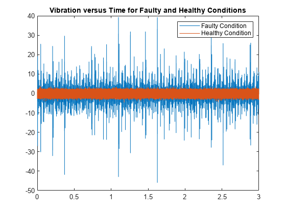
First, compare the inner and baseline time series directly using the same time-vector construction for the baseline1 data as previously for the inner1 data.
t_baseline1 = (0:length(x_baseline1)-1)/sr_baseline1;

figure
plot(t_inner1,x_inner1)
hold on
plot(t_baseline1,x_baseline1)
hold off
legend('Faulty Condition','Healthy Condition')
title('Vibration versus Time for Faulty and Healthy Conditions')
Calculate the second spectral moment of the baseline1 data. Compare the baseline1 and inner1 time histories.
[momentS_baseline1,t1_baseline1] = tfsmoment(x_baseline1,sr_baseline1,2);

figure
plot(t1_inner1,momentS_inner1)
hold on
plot(t1_baseline1,momentS_baseline1)
hold off
legend('Faulty Condition','Healthy Condition')
title('Second Spectral Moment versus Time for Faulty and Healthy Conditions')

The moment plot shows behavior different from the earlier vibration plot. The vibration data for the faulty case is much noisier with higher-magnitude spikes than for the healthy case, although both appear to be zero mean. However, the spectral variance (second spectral moment) is significantly lower for the faulty case. The moment of the faulty case is still more noisy than the healthy case.
Plot the histograms.
figure
histogram(momentS_inner1);
hold on
histogram(momentS_baseline1);
hold off
legend('Faulty Condition','Healthy Condition')
title('Second Spectral Moment for Faulty and Healthy Conditions')

The moment behaviors distinguish the faulty condition from the healthy condition in both plots. The histogram provides distinct distribution characteristics — center point along x-axis, spread, and peak histogram bin.
Determine the first four conditional spectral moments of a time-series data set, and extract the moments that you want to visualize with a histogram.
Load the data, which contains vibration measurements (x_inner1) and sample rate(sr_inner1) for machinery. Then use tfsmoment to compute the first four moments. These moments represent the statistical quantities of: 1) Mean; 2) Variance; 3) Skewness; and 4) Kurtosis.
You can specify the moment designators as a vector within the order argument.
load tfmoment_data.mat x_inner1 sr_inner1
momentS_inner1 = tfsmoment(x_inner1,sr_inner1,[1 2 3 4]);
Compare the dimensions of the input vector and the output matrix.
xsize = size(x_inner1)
xsize = 1×2

      146484           1
msize = size(momentS_inner1)
msize = 1×2

   524     4
The data vector x_inner is considerably longer than the vectors in the moment matrix momentS_inner1 because the spectrogram computation produces optimally-sized lower-resolution time windows. In this case, tfsmoment returns a moment matrix containing four columns, one column for each moment order.
Plot the histograms for the third (skewness) and fourth (kurtosis) moments. The third and fourth columns of momentS_inner1 provide these.
momentS_3 = momentS_inner1(:,3);
momentS_4 = momentS_inner1(:,4);
figure
histogram(momentS_3)
title('Third Spectral Moment (Skewness) of x inner1')
figure
histogram(momentS_4)
title('Fourth Spectral Moment (Kurtosis) of x inner1')
The plots are similar, but each has some unique characteristics with respect to number of bins and slope steepness.
By default, tfsmoment calls the function pspectrum internally to generate the power spectrogram that tfsmoment uses for the moment computation. You can also import an existing power spectrogram for tfsmoment to use instead. This capability is useful if you already have a power spectrogram as a starting point, or if you want to customize the pspectrum options by generating the spectrogram explicitly first.
Input a power spectrogram that has been generated with customized options. Compare the resulting spectral-moment histogram with one that tfsmoment generates using its pspectrum default options.
Load the data, which includes two power spectrums and the associated frequency and time vectors.
The p_inner1_def spectrum was created using the default pspectrum options. It is equivalent to what tfsmoment computes internally when an input spectrum is not provided in the syntax.
The p_inner1_MinThr spectrum was created using the MinThreshold pspectrum option. This option puts a lower bound on nonzero values to screen out low-level noise. For this example, the threshold was set to screen out noise below the 0.5% level.
load tfmoment_data.mat p_inner1_def f_p_def t_p_def ...
    p_inner1_MinThr f_p_MinThr t_p_MinThr
load tfmoment_data.mat x_inner1 x_baseline1
Determine the second spectral moments (variance) for both cases.
moment_p_def = tfsmoment(p_inner1_def,f_p_def,t_p_def,2);
moment_p_MinThr = tfsmoment(p_inner1_MinThr,f_p_MinThr,t_p_MinThr,2);
Plot the histograms together.
figure
histogram(moment_p_def);
hold on
histogram(moment_p_MinThr);
hold off
legend('Moment from Default P','Moment from Customized P')
title('Second Spectral Moment for Inner1 from Input Spectrograms')

The histograms have the same overall spread, but the thresholded moment histogram has a higher peak bin at a lower moment magnitude level than the default moment. This example is for illustration purposes only, but does show the impact that preprocessing in the spectrum computation stage can have.
By default, tfsmoment centralizes the moment as part of its calculation. That is, it subtracts the sensor-data mean (which is the first moment) from the sensor data as part of the Conditional Spectral Moments. If you want to preserve the offset, you can set the input argument Centralize to false.
Load the data, which contains vibration measurements x and sample rate sr for machinery. Calculate the 2nd moment (order = 2) both with centralization (default), and without centralization (Centralize = false). Plot the histograms together.
load tfmoment_data.mat x_inner1 sr_inner1
momentS_centr = tfsmoment(x_inner1,sr_inner1,2);
momentS_nocentr = tfsmoment(x_inner1,sr_inner1,2,'Centralize',false);

figure
histogram(momentS_centr)
hold on
histogram(momentS_nocentr);
hold off
legend('Centralized','Noncentralized')
title('Second Spectral Moment of x inner1 With and Without Centralization')

The noncentralized distribution is offset to the right.
Real-world measurements often come packaged as part of a time-stamped table that records actual time and readings rather than relative times. You can use the timetable format for capturing this data. This example shows how tfsmoment operates with a timetable input, in contrast to the data vector inputs used for the other tfsmoment examples, such as Plot the Conditional Spectral Moment of a Time Series Vector.
Load the data, which consists of a single timetable xt_inner1 containing measurement readings and time information for a piece of machinery. Examine the properties of the timetable.
load tfmoment_tdata.mat xt_inner1;
xt_inner1.Properties
ans =
  TimetableProperties with properties:

             Description: ''
                UserData: []
          DimensionNames: {'Time'  'Variables'}
           VariableNames: {'x_inner1'}
           VariableTypes: "double"
    VariableDescriptions: {}
           VariableUnits: {}
      VariableContinuity: []
                RowTimes: [146484×1 duration]
               StartTime: 0 sec
              SampleRate: 4.8828e+04
                TimeStep: 2.048e-05 sec
                  Events: []
        CustomProperties: No custom properties are set.
      Use addprop and rmprop to modify CustomProperties.
This table consists of columns for Time and the variables, where the only variable is x_inner1.
Find the second and fourth conditional spectral moments for the data in the timetable. Examine the properties of the resulting moment timetable.
order = [2 4];
momentS_xt_inner1 = tfsmoment(xt_inner1,order);
momentS_xt_inner1.Properties
ans =
  TimetableProperties with properties:

             Description: ''
                UserData: []
          DimensionNames: {'Time'  'Variables'}
           VariableNames: {'CentralSpectralMoment2'  'CentralSpectralMoment4'}
           VariableTypes: ["double"    "double"]
    VariableDescriptions: {}
           VariableUnits: {}
      VariableContinuity: []
                RowTimes: [524×1 duration]
               StartTime: 0.011725 sec
              SampleRate: 175.6403
                TimeStep: 0.0056935 sec
                  Events: []
        CustomProperties: No custom properties are set.
      Use addprop and rmprop to modify CustomProperties.
The returned timetable represents the moments in the variable 'CentralSpectralMoment2' and 'CentralSpectralMoment4', providing information not only on what specific moment was calculated, but also on whether it was centralized.
You can access the time and moment information directly from the timetable properties. Compute the second and fourth moments. Plot the fourth moment.
tt_inner1 = momentS_xt_inner1.Time;
momentS_inner1_2 = momentS_xt_inner1.CentralSpectralMoment2;
momentS_inner1_4 = momentS_xt_inner1.CentralSpectralMoment4;

figure
plot(tt_inner1,momentS_inner1_4)
title('Fourth Spectral Moment of Timetable Data')
As is illustrated in Plot the Conditional Spectral Moment of a Time Series Vector, a histogram is a very useful visualization for moment data. Plot the histogram, directly referencing the CentralSpectralMoment2 variable property.
figure
histogram(momentS_xt_inner1.CentralSpectralMoment2)
title('Second Spectral Moment of xt inner1 Timetable')
Input Arguments
Name-Value Arguments
Output Arguments
More About
References
[1] Loughlin, P. J. "What Are the Time-Frequency Moments of a Signal?" Advanced Signal Processing Algorithms, Architectures, and Implementations XI, SPIE Proceedings. Vol. 4474, November 2001.
[2] Loughlin, P., F. Cakrak, and L. Cohen. "Conditional Moment Analysis of Transients with Application to Helicopter Fault Data." Mechanical Systems and Signal Processing. Vol 14, Issue 4, 2000, pp. 511–522.
Extended Capabilities
Version History
Introduced in R2018a